Offensive eBPF - Part 2: Modern eBPF
by h3xduck
25 July 2025This is the second entry of the Offensive eBPF series. These were the previous entries:
Modern eBPF
We previously covered how classic BPF was born and how it looks like. But, since then, BPF has been greatly “extended” from basic network filtering, and so eBPF was born. In this post, I will cover anything there is to know about eBPF itself, and on the next one we will be ready for the fun security aspects ;)
Here is a list of most relevant eBPF features and when were they introduced:
| DESCRIPTION | KERNEL VERSION | YEAR |
|---|---|---|
| BPF: First addition in the kernel | 2.1.75 | 1997 |
| New JIT assembler | 3.0 | 2011 |
| eBPF: Added eBPF support | 3.15 | 2014 |
| New bpf() syscall | 3.18 | 2014 |
| Introduction of eBPF maps | 3.19 | 2015 |
| eBPF attached to kprobes | 4.1 | 2015 |
| Introduction of Traffic Control | 4.5 | 2016 |
| eBPF attached to tracepoints | 4.7 | 2016 |
| Introduction of XDP | 4.8 | 2016 |
The main breakthrough happened in the 3.15 kernel version, where Alexei Starovoitov, along with Daniel Borkmann, decided to expand the capabilities of BPF by remodelling the BPF instruction set and overall architecture. Anyways, here you can find the most comprehensive list of features (and is updated!) in eBPF. It’s my favourite source for checking out whether anything new has been introduced in the eBPF world :).
See below a figure I made describing the whole eBPF architecture:
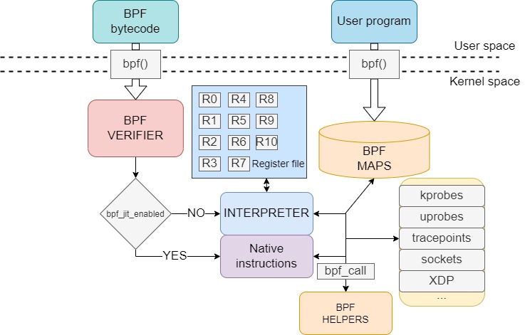
We are now going to go piece by piece explaining it :)
eBPF instruction set
The eBPF update included a complete remodel of the instruction set architecture (ISA) of the BPF VM. Therefore, eBPF programs will need to follow the new architecture in order to be interpreted as valid and executed.
| IMM | OFF | SRC | DST | OPCODE | |
|---|---|---|---|---|---|
| NUMBER OF BITS | 32 | 16 | 4 | 4 | 8 |
The table above shows the new instruction format for eBPF programs. As it can be observed, it is a fixed-length 64-bit instruction. The new fields are similar to x86_64 assembly, incorporating the typically found immediate and offset fields, and source and destination registers. Similarly, the instruction set is extended to be similar to the one typically found on x86_64 systems, the complete list can be consulted in the official documentation.
With respect to the classic BPF VM registers that we described in the previous post, they get extended from 32 to 64 bits of length, and the number of registers is incremented to 10, instead of the original accumulator and index registers. These registers are also adapted to be similar to those in assembly, see below:
| eBPF REGISTER | x86_64 REGISTER | PURPOSE |
|---|---|---|
| r0 | rax | Return value from functions and exit value of eBPF programs |
| r1 | rdi | Function call argument 1 |
| r2 | rsi | Function call argument 2 |
| r3 | rdx | Function call argument 3 |
| r4 | rcx | Function call argument 4 |
| r5 | r8 | Function call argument 5 |
| r6 | rbx | Callee saved register, value preserved between calls |
| r7 | r13 | Callee saved register, value preserved between calls |
| r8 | r14 | Callee saved register, value preserved between calls |
| r9 | r15 | Callee saved register, value preserved between calls |
| r10 | rbp | Frame pointer for stack, read only |
JIT Compilation
We have mentioned that eBPF registers and instructions describe an almost one-to-one correspondence to those in x86 assembly. This is in fact not a coincidence, but rather it is with the purpose of improving a functionality that was included in Linux kernel 3.0, called Just-in-Time (JIT) compilation. JIT compiling is an extra step that optimizes the execution speed of eBPF programs. It consists of translating BPF bytecode into machine-specific instructions, so that they run as fast as native code in the kernel. Machine instructions are generated during runtime, written directly into executable memory and executed there. Therefore, when using JIT compiling (a setting defined by the variable bpf_jit_enable, BPF registers are translated into machine-specific registers following their one-to- one mapping and bytecode instructions are translated into machine-specific instructions. There no longer exists an interpretation step by the BPF VM, since we can execute the code directly.
The eBPF verifier
One of the core elements in the whole eBPF architecture is the presence of the so-called eBPF verifier. Provided that we will be loading programs in the kernel from user space, these programs need to be checked for safety before being valid to be executed.
The verifier performs a series of tests which every eBPF program must pass in order to be accepted. Otherwise, user programs could leak privileged data, result in kernel memory corruption, or hang the kernel in an infinite loop, between others. Therefore, the verifier limits multiple aspects of eBPF programs so that they are restricted to the intended functionality, whilst at the same time offering a reasonable amount of freedom to the developer.
The following are the most relevant checks that the verifier performs in eBPF programs:
- Tests for ensuring overall control flow safety:
- No loops allowed (bounded loops accepted since kernel version 5.3).
- Function call and jumps safety to known, reachable functions. = Sleep and blocking operations not allowed (to prevent hanging the kernel).
- Tests for individual instructions:
- Divisions by zero and invalid shift operations.
- Invalid stack access and invalid out-of-bound access to data structures.
- Reads from uninitialized registers and corruption of pointers.
These checks are performed by two main algorithms:
- Build a graph representing the eBPF instructions. Check that it is in fact a direct acyclic graph (DAG), meaning that the verifier prevents loops and unreachable instructions.
- Simulate execution flow by starting on the first instruction and following each possible path, observing at each instruction the state of every register and of the stack.
eBPF maps
Where do eBPF programs save their data? The answer is on an eBPF map. An eBPF map is a generic storage for eBPF programs used to share data between user and kernel space, to maintain persistent data between eBPF calls and to share information between multiple eBPF programs.
A map consists of a key + value tuple. Both fields can have an arbitrary data type, the map only needs to know the length of the key and the value field at its creation. Programs can open maps by specifying their ID, and lookup or delete elements in the map by specifying its key, also insert new ones by supplying the element value and they key to store it with.
Creating a map requires a struct with the following fields:
| Field | Value |
|---|---|
| type | Type of eBPF map. Described in Table 2.6 |
| key_size | Size of the data structure to use as a key |
| value_size | Size of the data structure to use as value field |
| max_entries | Maximum number of elements in the map |
And the following are the main types of eBPF maps available for use:
| Type | Description |
|---|---|
| BPF_MAP_TYPE_HASH | A hash table-like storage where elements are saved as key-value pairs (tuples). |
| BPF_MAP_TYPE_ARRAY | Stores elements in a simple array, allowing direct lookup by index. |
| BPF_MAP_TYPE_RINGBUF | Acts as a ring buffer for sending notifications from the kernel to user space. |
| BPF_MAP_TYPE_PROG_ARRAY | Holds references (descriptors) to eBPF programs, useful for program chaining. |
The eBPF ring buffer
Your eBPF programs may have a in-kernel part and one executing in the userspace. How do they communicate? The answer is with the ring buffer. These are a special kind of eBPF maps, providing a one-way directional communication system, going from an eBPF program in the kernel to a user space program that subscribes to its events.
The bpf() syscall
The bpf() syscall is used to issue commands from user space to kernel space in eBPF programs. This syscall can perform a great range of actions, changing its behaviour depending on the parameters, here are the most important ones:
| COMMAND | ATTRIBUTES | DESCRIPTION |
|---|---|---|
| BPF_MAP_CREATE | Struct with map info as defined in Table 2.5 | Create a new map |
| BPF_MAP_LOOKUP_ELEM | Map ID, and struct with key to search in the map | Get the element on the map with a specific key |
| BPF_MAP_UPDATE_ELEM | Map ID, and struct with key and new value | Update the element of a specific key with a new value |
| BPF_MAP_DELETE_ELEM | Map ID and struct with key to search in the map | Delete the element on the map with a specific key |
| BPF_PROG_LOAD | Struct describing the type of eBPF program to load | Load an eBPF program into the kernel |
For BPF_PROG_LOAD, these are the most common types of eBPF programs to load (but don’t worry, we’ll go over them later one by one):
| Program Type | Description |
|---|---|
| BPF_PROG_TYPE_KPROBE | Program to instrument code attached to a kprobe |
| BPF_PROG_TYPE_UPROBE | Program to instrument code attached to a uprobe |
| BPF_PROG_TYPE_TRACEPOINT | Program to instrument code at a syscall tracepoint |
| BPF_PROG_TYPE_XDP | Program to filter, redirect, and monitor network events from the Xpress Data Path (XDP) |
| BPF_PROG_TYPE_SCHED_CLS | Program to filter, redirect, and monitor events using the Traffic Control classifier |
eBPF helpers
Our last component to cover of the eBPF architecture are the eBPF helpers. Since eBPF programs have limited accessibility to kernel functions (which kernel modules commonly have free access to), the eBPF system offers a set of limited functions called helpers, which are used by eBPF programs to perform certain actions and interact with the context on which they are run. The list of helpers a program can call varies between eBPF program types, since different programs run in different contexts.
It is important to highlight that, just like commands issued via the bpf() syscall can only be issued from the user space, eBPF helpers correspond to the kernel-side of eBPF program exclusively. Note that we will also find a symmetric correspondence to those functions of the bpf() syscall related to map operations (since these are accessible both from user and kernel space).
| eBPF Helper | Description |
|---|---|
| bpf_map_lookup_elem() | Query an element with a certain key in a map |
| bpf_map_delete_elem() | Delete an element with a certain key in a map |
| bpf_map_update_elem() | Update the value of the element with a certain key in a map |
| bpf_probe_read_user() | Attempt to safely read data at a specific user address into a buffer |
| bpf_probe_read_kernel() | Attempt to safely read data at a specific kernel address into a buffer |
| bpf_trace_printk() | Like printk() in kernel modules, writes buffer in /sys/kernel/debug/tracing/trace_pipe |
| bpf_get_current_pid_tgid() | Get the process’s Process Id (PID) and thread group id (TGID) |
| bpf_get_current_comm() | Get the name of the executable |
| bpf_probe_write_user() | Attempt to write data at a user memory address |
| bpf_override_return() | Override the return value of a probed function |
| bpf_ringbuf_submit() | Submit data to a specific eBPF ring buffer and notify subscribers |
| bpf_tail_call() | Jump to another eBPF program while preserving the current stack |
eBPF program types
We have briefly commented that there are different types of eBPF programs available. Here are the most interesting ones:
XDP
Express Data Path (XDP) programs are a novel type of eBPF program that allows for the lowest-latency traffic filtering and monitoring in the whole Linux kernel. In order to load an XDP program, a bpf() syscall with the command BPF_PROG_LOAD and the program type BPF_PROG_TYPE_XDP must be issued. These programs are directly attached to the Network Interface Controller (NIC) driver, and thus they can process the packet before any other module.
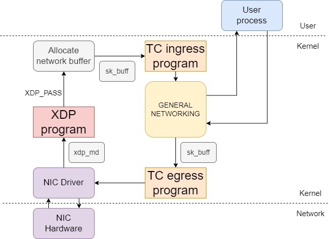
The image above shows how XDP is integrated in the network processing of the Linux kernel. After receiving a raw packet (in the figure, xdp_md, which consists on the raw bytes plus some very basic metadata about the packet) from the incoming traffic, XDP program can perform the following actions:
- Analyze the data between the packet buffer bounds.
- Modify the packet contents, and modify the packet length.
- Decide between one of the actions displayed below:
| Action | Description |
|---|---|
| XDP_PASS | Let the packet proceed, keeping any modifications made to it. |
| XDP_TX | Send the packet back out through the same network interface (NIC) it came in on, with modifications. |
| XDP_DROP | Drop the packet completely; the kernel’s networking stack will not be notified about this packet. |
These programs also have some XDP-exclusive eBPF helpers:
| eBPF Helper | Description |
|---|---|
| bpf_xdp_adjust_head() | Enlarges or reduces the size of a packet by moving the address of its first byte. |
| bpf_xdp_adjust_tail() | Enlarges or reduces the size of a packet by moving the address of its last byte. |
Traffic Control
Traffic Control (TC) programs are also indicated for networking instrumentation. Similarly to XDP, their module is positioned before entering the overall network processing of the kernel. But as we saw in the prior image, there are some difference aspects:
- TC programs receive a network buffer with metadata (sk_buff) about the packet in it. This renders TC programs less ideal than XDP for performing large packet modifications (like new headers), but at the same time the additional metadata fields make it easier to locate and modify specific packet fields.
- TC programs can be attached to the ingress or egress points, meaning that an eBPF program can operate not only over incoming traffic, but also over the outgoing packets.
With respect to how TC programs operate, the Traffic Control system in Linux is greatly complex and would require a complete section by itself. In fact, it was already a complete system before the appearance of eBPF. Full documentation can be found here. For this document, we will explain the overall process needed to load a TC program (this is a great source for getting to know this):
- The TC program defines a so-called queuing discipline (qdisc), a packet scheduler that issues packets in a First-In-First-Out (FIFO) order as soon as they are received. This qdisc will be attached to a specific network interface (e.g.: wlan0).
- Our TC eBPF program is attached to the qdisc. It will work as a filter, being run for every of the packets dispatched by the qdisc.
Similarly to XDP, the TC eBPF programs can decide an action to be executed on a packet by specifying a return value. These actions are almost analogous to the ones in XDP:
| Action | Description |
|---|---|
| TC_ACT_OK | Let the packet proceed, keeping any modifications made to it. |
| TC_ACT_RECLASSIFY | Return the packet to the back of the qdisc (queueing discipline) scheduling queue for further processing. |
| TC_ACT_SHOT | Drop the packet completely; the kernel’s networking stack will not be notified about this packet. |
Finally, as in XDP, there exists a list of useful BPF helpers:
| eBPF Helper | Description |
|---|---|
| bpf_l3_csum_replace() | Recomputes the network layer 3 (for example, IP) checksum of the packet. |
| bpf_l4_csum_replace() | Recomputes the network layer 4 (for example, TCP) checksum of the packet. |
| bpf_skb_store_bytes() | Writes a data buffer into the packet. |
| bpf_skb_pull_data() | Reads a sequence of packet bytes into a buffer. |
| bpf_skb_change_head() | (Only) enlarges the size of a packet by moving the address of its first byte. |
| bpf_skb_change_tail() | Enlarges or reduces the size of a packet by moving the address of its last byte. |
Tracepoints
Tracepoints are a technology in the Linux kernel that allows to hook functions in the kernel, connecting a ‘probe’: a function that is executed every time the hooked function is called. These tracepoints are set statically during kernel development, meaning that for a function to be hooked, it needs to have been previously marked with a trace- point statement indicating its traceability. At the same time, this limits the number of tracepoints available.
The list of tracepoint events available depends on the kernel version and can be visited
under the directory /sys/kernel/debug/tracing/events.
It is particularly relevant for our later research that most of the system calls incorporate
a tracepoint, both when they are called (enter tracepoint) and when they are exited (exit
tracepoints). This means that, for a system call sys_open, both the tracepoint sys_enter_open and sys_exit_open are available.
Also, note that the probe functions that are called when hitting a tracepoint receive
some parameters related to the context on which the tracepoint is located. In the case
of syscalls, these include the parameters with which the syscall was called (only for enter syscalls, exit ones will only have access to the return value). The exact parameters
and their format which a probe function receives can be visited in the file /sys/kernel/debug/tracing/events/<subsystem>/<tracepoint>/format.
In the previous example with sys_enter_open, this is /sys/kernel/debug/tracing/events/syscalls/sys_enter_open/format.
In eBPF, a program can issue a bpf() syscall with the command BPF_PROG_LOAD
and the program type BPF_PROG_TYPE_TRACEPOINT, specifying which is the function with the tracepoint to attach to and an arbitrary function probe to call when it is hit.
This function probe is defined by the user in the eBPF program submitted to the kernel.
Kprobes
Kprobes are another tracing technology of the Linux kernel whose functionality has been become available to eBPF programs. Similarly to tracepoints, kprobes enable to hook functions in the kernel, with the only difference that it is dynamically attached to any arbitrary function, rather than to a set of predefined positions. It does not require that kernel developers specifically mark a function to be probed, but rather kprobes can be attached to any instruction, with a short list of blacklisted exceptions.
As it happened with tracepoints, the probe functions have access to the parameters
of the original hooked function. Also, the kernel maintains a list of kernel symbols (ad-
dresses) which are relevant for tracing and that offer us insight into which functions we
can probe. It can be visited under the file /proc/kallsyms, which exports symbols of kernel
functions and loaded kernel modules.
Also similarly, since tracepoints could be found in their enter and exit variations, kprobes have their counterpart, named kretprobes, which call the hooked probe once a return instruction is reached after the hooked symbol. This means that a kretprobe hooked to a kernel function will call the probe function once it exits.
In eBPF, a program can issue a bpf() syscall with the command BPF_PROG_LOAD
and the program type BPF_PROG_TYPE_KPROBE, specifying which is the function
with the kprobe to attach to and an arbitrary function probe to call when it is hit. This
function probe is defined by the user in the eBPF program submitted to the kernel.
Uprobes
Uprobes is the last of the main tracing technologies which has been become accessible to eBPF programs. They are the counterparts of Kprobes, allowing for tracing the execution of an specific instruction in the user space, instead of in the kernel. When the execution flow reaches a hooked instruction, a probe function is run.
For setting an uprobe on a specific instruction of a program, we need to know three components:
- The name of the program.
- The address of the function where the instruction is contained.
- The offset at which the specific instruction is placed from the start of the function.
Similarly to kprobes, uprobes have access to the parameters received by the hooked function. Also, the complementary uretprobes exist too, running the probe function once the hooked function returns.
In eBPF, programs can issue a bpf() syscall with the command BPF_PROG_LOAD
and the program type BPF_PROG_TYPE_UPROBE, specifying the function with the
uprobe to attach to and an arbitrary function probe to call when it is hit. This function
probe is also defined by the user in the eBPF program submitted to the kernel
Developing eBPF programs
For an eBPF developer, programming bytecode and working with bpf() calls natively is not an easy task, therefore an additional layer of abstraction was needed.
Nowadays, there exists multiple popular alternatives for writing and running eBPF programs. We will overview which they are and proceed to analyse in further detail the option that we will use for the development of our rootkit.
BCC
BPF Compiler Collection (BCC) is one of the first and well-known toolkits for eBPF programming available. It allows to include eBPF code into user programs. These programs are developed in Python, and the eBPF code is embedded as a plain string.
Although BCC offers a wide range of tools to easy the development of eBPF programs, I personally find it not to be the most appropriate for our large-scale eBPF project. In particular, this is because eBPF programs are stored as a python string, which leads to difficult scalability, poor development experience given that programming errors are detected at runtime (once the python program issues the compilation of the string), and simply better features from competing libraries.
Bpftool
Bpftool is not a development framework like BCC, but one of the most relevant tools for eBPF program development. Some of its functionalities include:
- Loading eBPF programs.
- List running eBPF programs.
- Dumping bytecode from live eBPF programs.
- Extract program statistics and data from programs.
- List and operate over eBPF maps.
Although we will not be covering bpftool during our the rest of my posts, it is one of the best tools out there (together with bpftrace) and is a key tool for debugging eBPF programs, particularly to peek data at eBPF maps during runtime.
Libbpf
This is my recommended way of developing big eBPF projects. Libbpf is a library for loading and interacting with eBPF programs, which is currently maintained in the Linux kernel source tree. It is one of the most popular frameworks to develop eBPF applications, both because it makes eBPF programming similar to com- mon kernel development and because it aims at reducing kernel-version dependencies, thus increasing programs portability between systems.
As we discussed, eBPF programs are composed of both the eBPF code in the kernel and a user space program that can interact with it. With libbpf, the eBPF kernel program is developed in C (a real program, not a string later compiled as with BCC), while user programs are usually developed in C, Rust or GO. For TripleCross, I used the C version of libbpf, so both the user and kernel side of our rootkit will be developed in this language.
When using libbpf with the C language, both the user-side and kernel eBPF program are compiled together using the Clang/LLVM compiler, translating C instructions into eBPF bytecode.
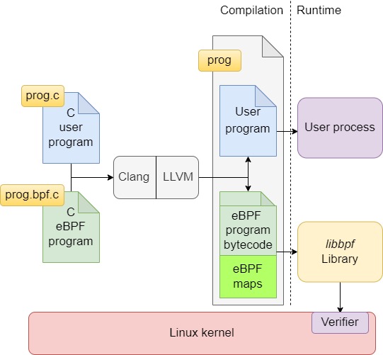
As it can be observed in the image above, the result of the compilation is a single program, comprising the user-side which will launch a user process, the eBPF bytecode to be run in the kernel, and other structures libbpf generates about eBPF maps and other meta data. This program is encapsulated as a single ELF file.
One of the main functionalities of libbpf to simplify eBPF programming is the BPF skeleton. This is auto-generated code by libbpf whose aim is to simplify working with eBPF from the user-side program. As a summary, it parses the eBPF programs developed (which may be using different technologies such as XDP, kprobes, TC…) and the eBPF maps used, and as a result offers a simple set of functions for dealing with these programs from the user program. For example, it allows for loading and unloading a specific eBPF program from user space at runtime, but also other things:
| Function Name | Description |
|---|---|
| Parses the eBPF programs and maps. | |
| Loads the eBPF map into the kernel after validation and creates the maps, but the programs are not active yet. | |
| Activates the eBPF programs by attaching them to the relevant parts of the kernel (e.g., kprobes to functions). | |
| Detaches and unloads the eBPF programs from the kernel. |
(Note that
Wrapping up
And that’s all to know about modern eBPF! Next, we will start covering some of the basic security features embedded in eBPF. See you on the next entry of the eBPF series:
Part 3 (Yet to come!)
tags:
This work is licensed under a Creative Commons Attribution 4.0 International License.